python实现一维二维梯度下降法

梯度下降法是机器学习场景的算法，其核心为求最小值。

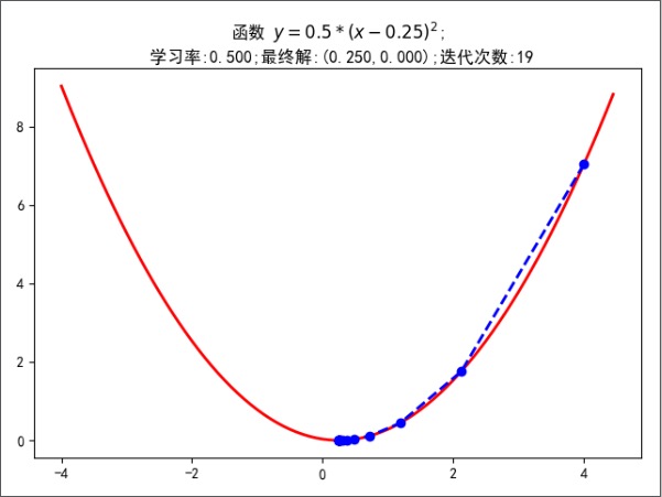
y=x2函数求解最小值，最终解为 x=0.00 y=0.00

一维元素图像

# 构建一维元素图像，开口向上
import numpy as np
import matplotlib.pyplot as plt
import matplotlib as mpl

mpl.rcParams['font.family'] = 'sans-serif'
mpl.rcParams['font.sans-serif'] = 'SimHei'
mpl.rcParams['axes.unicode_minus'] = False


def f1(x):
    return 0.5 * (x - 0.25) ** 2  # 平方


# 一阶导数
def h1(x):
    return 0.5 * 2 * (x - 0.25)


# 使用梯度下降法进行解答
GD_X = []
GD_Y = []
x = 4
alpha = 0.5  # 学习步长，也叫阿尔法
f_change = f1(x)  # 得到y0的值
f_current = f_change  # y0当前值
GD_X.append(x)
GD_Y.append(f_current)

# 迭代次数
iter_number = 0

while f_change > 1e-10 and iter_number < 100:
    iter_number += 1
    x = x - alpha * h1(x)
    tmp = f1(x)
    # 判断y值的变化，不能太小
    f_change = np.abs(f_current - tmp)
    f_current = tmp
    GD_X.append(x)
    GD_Y.append(f_current)

print(u'最终的结果:(%.5f,%.5F)' % (x, f_current))
print(u'迭代次数: %d' % iter_number)
print(GD_X)

# 构建数据
X = np.arange(-4, 4.5, 0.05)
Y = np.array(list(map(lambda t: f1(t), X)))

# 画图
plt.figure(facecolor='w')
plt.plot(X, Y, 'r-', linewidth=2)
plt.plot(GD_X, GD_Y, 'bo--', linewidth=2)
plt.title(u'函数 $y=0.5*(x-0.25)^2$;\n 学习率:%.3f;最终解:(%.3f,%.3f);迭代次数:%d' % (alpha, x, f_current, iter_number))
plt.show()

运行结果：

最终的结果:(0.25001,0.00000)
迭代次数: 19
[4, 2.125, 1.1875, 0.71875, 0.484375, 0.3671875, 0.30859375, 0.279296875, 0.2646484375, 0.25732421875, 0.253662109375, 0.2518310546875, 0.25091552734375, 0.250457763671875, 0.2502288818359375, 0.25011444091796875, 0.2500572204589844, 0.2500286102294922, 0.2500143051147461, 0.25000715255737305]

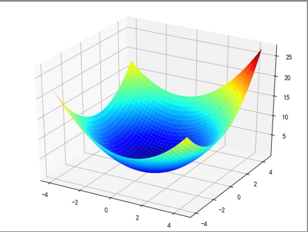
二维

import numpy as np
import matplotlib.pyplot as plt
import matplotlib as mpl
from mpl_toolkits.mplot3d import Axes3D

mpl.rcParams['font.family'] = 'sans-serif'
mpl.rcParams['font.sans-serif'] = 'SimHei'
mpl.rcParams['axes.unicode_minus'] = False


# 二维原始图像
def f2(x, y):
    return 0.6 * (x + y) ** 2 - x * y


# 导函数、偏导
def hx2(x, y):
    return 0.6 * 2 * (x + y) - y


def hy2(x, y):
    return 0.6 * 2 * (x + y) - x


# 使用梯度下降法进行求解
GD_X1 = []
GD_X2 = []
GD_Y = []
x1 = 4
x2 = 4
alpha = 0.5  # 学习步长，也叫阿尔法
f_change = f2(x1, x2)  # 得到y0的值
f_current = f_change  # y0当前值
GD_X1.append(x1)
GD_X2.append(x2)
GD_Y.append(f_current)
iter_number = 0

while f_change > 1e-10 and iter_number < 100:
    iter_number += 1
    prex1 = x1
    prex2 = x2
    x1 = x1 - alpha * hx2(prex1, prex2)
    x2 = x2 - alpha * hy2(prex1, prex2)
    tmp = f2(x1, x2)
    # 判断y值的变化，不能太小
    f_change = np.abs(f_current - tmp)
    f_current = tmp
    GD_X1.append(x1)
    GD_X2.append(x2)
    GD_Y.append(f_current)

print(u'最终的结果:(%.5f,%.5f,%.5f)' % (x1, x2, f_current))
print(u'迭代过程中X的取值，迭代次数: %d' % iter_number)
print(GD_X1)

# 构建数据
X1 = np.arange(-4, 4.5, 0.2)
X2 = np.arange(-4, 4.5, 0.2)

X1, X2 = np.meshgrid(X1, X2)

Y = np.array(list(map(lambda t: f2(t[0], t[1]), zip(X1.flatten(), X2.flatten()))))
Y.shape = X1.shape

# 画图
fig = plt.figure(facecolor='w')
ax = Axes3D(fig)
ax.plot_surface(X1, X2, Y, rstride=1, cstride=1, cmap=plt.cm.jet)
ax.plot(GD_X1, GD_X2, GD_Y, 'bo--', linewidth=1)
plt.show()

运行结果

最终的结果:(0.00000,0.00000,0.00000)
迭代过程中X的取值，迭代次数: 12
[4, 1.2000000000000002, 0.3600000000000001, 0.10800000000000004, 0.03240000000000001, 0.009720000000000006, 0.002916000000000002, 0.0008748000000000007, 0.0002624400000000003, 7.873200000000009e-05, 2.3619600000000034e-05, 7.0858800000000115e-06, 2.125764000000004e-06]